
categories: physics, automation & robotics, mechanics
Bonus post in the series, since this is the question that actually kicked off a lot of the earlier posts: if you're building a pick-and-place robot arm, how do you know which motor and gearbox to buy for the joint? The analogy is simple — hold a heavy dumbbell out at arm's length. Your arm resists two things: its own weight fighting gravity (a constant drag, even if you don't move at all), and the extra effort it takes to actually accelerate the weight upward quickly (fighting inertia). A joint motor has to overcome exactly those same two things at once, and this post walks through sizing one for real numbers.
Worked example: torque for a pick-and-place arm joint
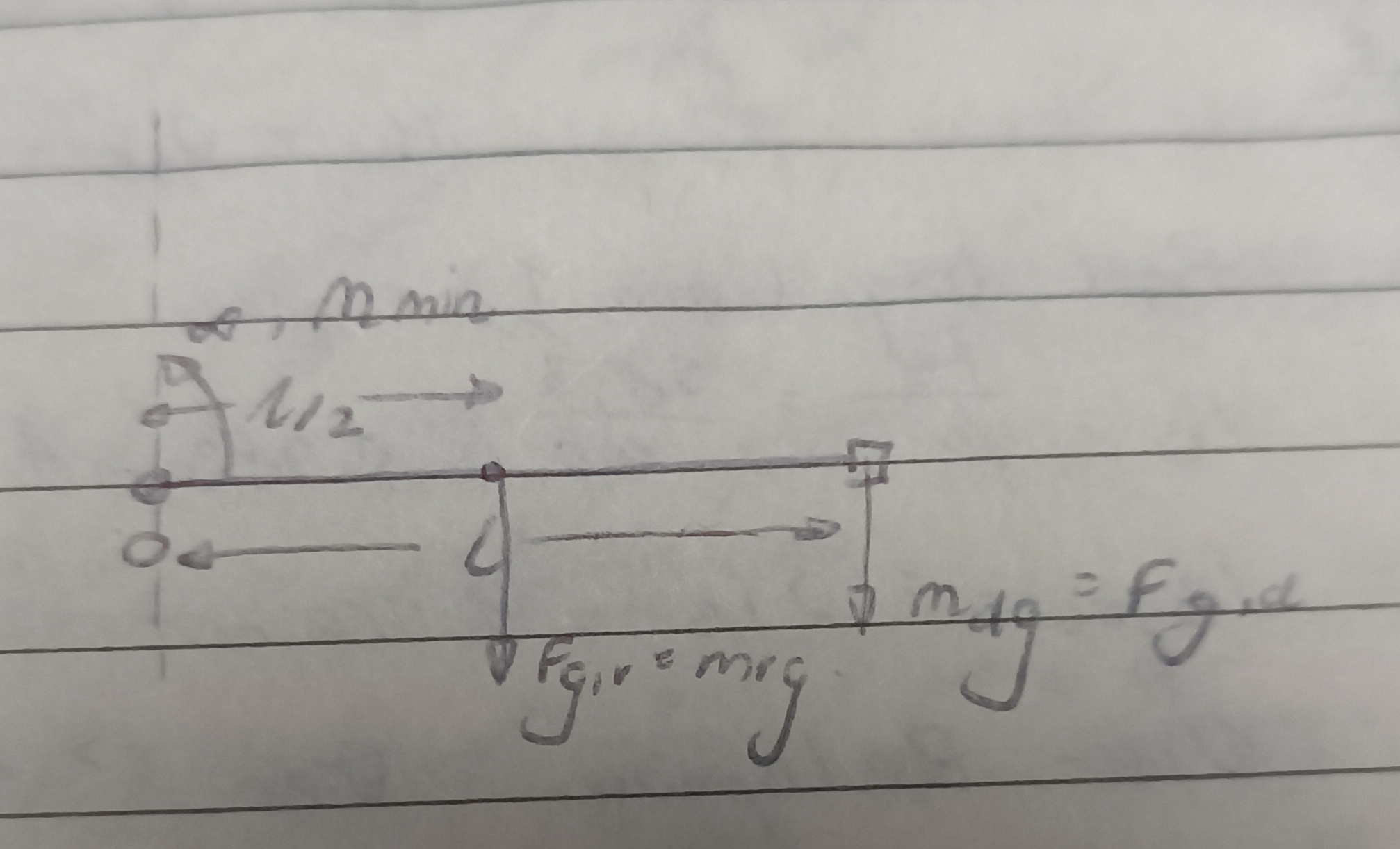
Setup: you're designing the drive for a single joint of a pick-and-place robot arm, rotating in a vertical plane. The arm has to be able to start moving abruptly from the horizontal position — the worst case, since that's where gravity's leverage on the joint is largest.
Data: the arm itself is modeled as a uniform thin rod pivoting about its end, mass $$m_r = 2\ \text{kg}$$, length $$L = 0.6\ \text{m}$$. The part being carried in the gripper is modeled as a point mass at the very tip of the arm, $$m_d = 1.5\ \text{kg}$$. The joint starts from rest and must reach an angular velocity of $$\omega = 4\ \text{rad/s}$$ within $$t = 0.2\ \text{s}$$, at constant angular acceleration. $$g = 9.81\ \text{m/s}^2$$.
Step 1 — total moment of inertia. Moment of inertia is rotational inertia's answer to mass: it measures how much a body resists a change in its rotational speed. The arm rotates about its own end (rod formula $$I = \frac{1}{3}mL^2$$), and the payload sits as a point mass at distance $$L$$ from the pivot ($$I = mL^2$$): $$I_{arm} = \frac{1}{3}m_r L^2 = \frac{1}{3}\cdot2\cdot(0.6)^2 = 0.24\ \text{kg}\cdot\text{m}^2$$ $$I_{payload} = m_d L^2 = 1.5\cdot(0.6)^2 = 0.54\ \text{kg}\cdot\text{m}^2$$ $$I_{tot} = I_{arm} + I_{payload} = 0.24+0.54 = 0.78\ \text{kg}\cdot\text{m}^2$$
Step 2 — required angular acceleration. Straight from the definition of constant angular acceleration, going from rest to $$\omega$$ over the ramp-up time $$t$$: $$\alpha = \frac{\Delta\omega}{\Delta t} = \frac{\omega-\omega_0}{t} = \frac{4-0}{0.2} = 20\ \text{rad/s}^2$$
Step 3 — gravitational (static) torque. This is the torque the motor has to supply just to hold the arm up, before it even starts moving — it's largest exactly at the horizontal position, since that's where the weight's moment arm about the joint is longest. The arm's own weight acts at its center of mass ($$L/2$$); the payload's weight acts at the full length $$L$$: $$M_{g,arm} = m_r\cdot g\cdot\frac{L}{2} = 2\cdot9.81\cdot0.3 = 5.886\ \text{N}\cdot\text{m}$$ $$M_{g,payload} = m_d\cdot g\cdot L = 1.5\cdot9.81\cdot0.6 = 8.829\ \text{N}\cdot\text{m}$$ $$M_g = M_{g,arm}+M_{g,payload} = 5.886+8.829 = 14.715\ \text{N}\cdot\text{m}$$
Step 4 — dynamic torque. On top of just holding the arm level, the motor has to supply extra torque to actually accelerate the whole assembly — the rotational equivalent of $$F=ma$$: $$M_d = I_{tot}\cdot\alpha = 0.78\cdot20 = 15.6\ \text{N}\cdot\text{m}$$
Step 5 — minimum motor torque. Both effects act in the same direction during a horizontal start-up, so they simply add: $$M_{min} = M_g + M_d = 14.715+15.6 = 30.315\ \text{N}\cdot\text{m} \approx 30.32\ \text{N}\cdot\text{m}$$ In practice you'd then pick a motor+gearbox combination whose continuous/peak torque at the output shaft clears this number with some margin, exactly the same overdrive-factor logic used for the transistor base resistor in the previous post — never design right at the calculated minimum.
This is the same two-term pattern you'll see in basically every actuator-sizing problem: a static/gravitational term that doesn't care how fast you're moving, plus a dynamic/inertial term that only shows up when you're accelerating. Work out both separately, add them, and you have your minimum spec. Thank you for reading! Next post: solving kinematics problems where acceleration depends on velocity, using differential equations.
Read more